Project Sample: A Presidency of Protest

In “A Presidency of Protest,” I use data from countlove’s web scraper to visualize protests during the first two years of Donald Trump’s presidency. News stories about protests are scraped every day before being cleaned and tagged by the project’s creators, Tommy Leung and Nathan Perkins. I analyzed the data and created initial visualizations in R, and then polished the visualizations in Illustrator.

This project sample shows the code used to create a chart of protests related to gun control and then the polished product. Code is also included for an animated GIF that will be used for promotion on social media.

DATA Preparation

The dataset is clean and tidy upon download:

A quick audit of the data showed four potential challenges:

Not all protests have attendee information
The event type and tagging system changed in January 2019, so the most recent protests do not have event types
Tags for each event are concatenated together in a single field
The tagging is correct, but not completely consistent: one protest might have “Civil Rights; For Planned Parenthood” as tags, while a similar protest might have “For abortion rights; For women’s rights.”

I decided to focus on the number of protests, rather than the number of people attending those protests. Since the tagging system was a little inconsistent, I used both event type and tags to group protests together. To untangle the tags, I used Andrew Ba Tran’s muckrakr package. Muckrakr created a field for each tag with a 1 for every protest that used the tag.

First, I loaded the necessary packages and read in the data. Muckrakr isn’t yet on CRAN and must be installed from Github:

install.packages("devtools")
library(devtools)
install_github("andrewbtran/muckrakr")

library(tidyerse)
library(muckrakr)
library(lubridate)
library(gganimate)
library(gifski)
library(maps)
library(mapdata)
library(mapproj)

protests <- read.csv("protests.csv", header=TRUE)

I conducted a quick audit of the data to make sure that tags and events matched the linked news stories:

psamp <- base::sample(1:nrow(protests), 30)
audit <- protests[psamp,]
write.csv(audit, "protestaudit.csv")

Once I was satisfied that the tags and event types were accurate, I moved on to formatting the data. I filtered the data to the first two years of Trump’s presidency and added fields for week and week rank. Weeks run from Monday to Sunday so that the events of a continuous weekend are grouped together in one week:

protests$date <- as.Date(protests$date)
protests <- filter(protests, date >= "2017-01-20", 
    date <="2019-01-19")
protests <- mutate(protests, week=as.Date(cut(date, 
    breaks="week", starts.on.monday=TRUE)))
protests <- mutate(protests, weekrank = dense_rank(week), 
    group = 1, group = 1:nrow(protests))

Finally, I untangled the tags field into a series of columns:

tags <- untangle(data=protests, x="tags", pattern="[;]", 
    verbose=TRUE)

Data Exploration

I explored the tags and event types to choose which subjects to explore. My final six subjects were gun control, immigration, healthcare, the Women’s March, the Russia investigation, and Supreme Court nominees. Exploring the data was an iterative and extensive process, so I’ll show a couple of examples of how I searched for gun control-related protests.

I looked at which specific weeks had large numbers of protests, and then which event types were common on those days. That gave me the names of some event types related to gun control:

top_week <- protests %>% group_by(week) %>% 
    summarise(count = n()) %>% 
    arrange(desc(count))
top_week <- mutate(top_week, rank = min_rank(desc(count)))
week_10 <- filter(top_week, rank <=10)
week_10_protests <- protests %>% 
    filter(week %in% week_10$week) %>% 
    group_by(week, event) %>% 
    summarise(count=n()) %>% 
    arrange(week)

From there, I looked at which tags were used with gun-control-related event types:

tags %>% filter(event == "Guns (March for Our Lives)") %>% 
     select(14:422) %>% 
     lapply(sum) %>% 
     as.data.frame() %>% 
     t() %>% 
     as.data.frame() %>% 
     tibble::rownames_to_column() %>% filter(V1>0) %>%
     arrange(desc(V1))

And then looked at other events associated with those tags:

tags %>% filter(for_greater_gun_control == 1) %>% 
    group_by(event) %>% 
    summarise(count = n()) %>% 
    arrange(desc(count))

Once I was sure that I had all of the relevant tags and events, I created a field to “bucket” all of the protests related to gun control:

tags <- mutate(tags, GunControlBucket = ifelse(event %in% c("Guns 
    (National Walkout Day)", "Guns", "Guns (March For Our
    Lives)", "Guns (Second Amendment)", "Guns (Counter
    Protest)",  "Guns (Wear Orange)", "Guns (NRA)", "Guns (Second 
    Amendment; Counter Protest)", "Guns (Violence)","Guns 
    (Invited Speaker)") | guns ==1 | for_greater_gun_control ==1 
    | against_greater_gun_control == 1, 1, 0))

Then I created a table with the count of gun control protests per week:

allWeekCount <- tags %>% group_by(week,weekrank) %>% 
    summarise(GunControl = sum(GunControlBucket)

Data Visualization: Gun Control

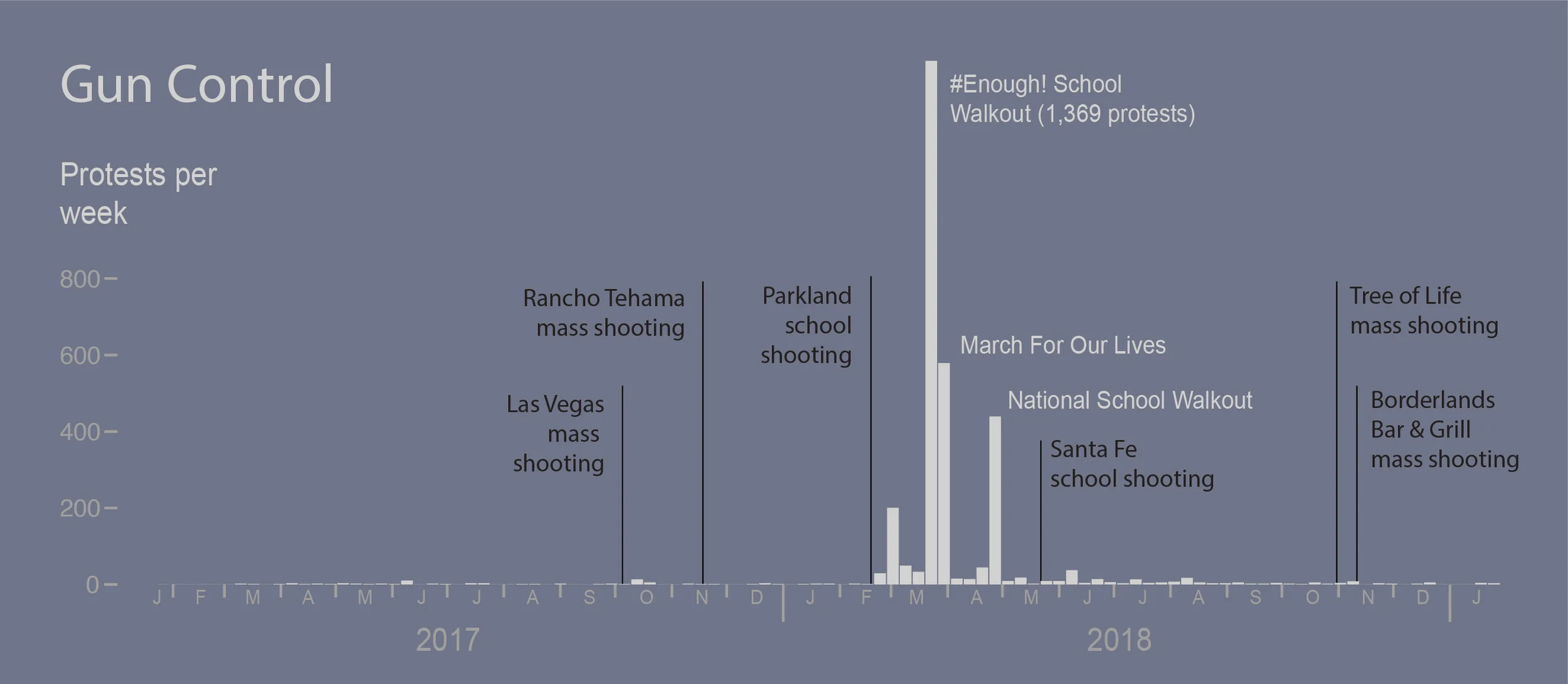
In addition to visualizing protests per week, I also wanted to mark the dates of mass shootings on the graph. I decided to place the events on the graph in R, rather than trying to manually add them in Illustrator, so that I could make sure they were accurately located on the chart.

I created a list of mass shootings and read it into R. Then I took the difference between each date and 1/16/17 (the beginning of the first week of Trump’s presidency) and divided that by seven. That gave me the precise location of each event in the chart, because the X axis would be graphed by each week’s rank from 1 to 105:

eventdates <- read.csv("event dates.csv")
eventdates <- mutate(eventdates, Date = as.Date(Date,'%m/%d/%y'), 
    mark = (Date - as.Date("2017-01-16"))/7)

I followed a similar process to mark the first day of each month on the X axis:

monthbreak <- read.csv("monthbreaks.csv")
monthbreak <- mutate(monthbreak, Date = as.Date(Date,'%m/%d/%y'),
   mark = (Date - as.Date("2017-01-16"))/7)

Finally, I wrote the code for the graph itself. The ggplot code is extensive: in the final project, I have six matching bar charts, so I wanted to minimize the number of manual edits required in Illustrator. The geom_vline section in the code places vertical lines when each of the events took place. The breaks argument in scale_x_continuous places tick marks at the transition points between months:

ggplot(allWeekCount, aes(x=weekrank, y=GunControl), width=.25) + 
    geom_vline(xintercept = eventdates[eventdates$Category == 
       "GunControl",]$mark, size=.25, color = "#9baec1") + 
    geom_bar(stat='identity', fill="#D1D1D1") + 
    theme(panel.grid.major = element_blank(), 
        panel.grid.minor =  element_blank(), 
        panel.background = element_blank(), 
        plot.background = element_rect(fill = "#707589”), 
        axis.text.x = element_text(colour="#A0A0A0"), 
        axis.text.y = element_text(colour="#A0A0A0"), 
        axis.ticks = element_line(color="#A0A0A0"), 
        axis.ticks.length=unit(5, "points")) + 
    labs(x="Gun Control", y="") + 
    scale_y_continuous(expand = c(0,0), breaks = c(0, 200, 400, 
        600, 800, 1000, 1200, 1400), limits = c(0, 1400)) + 
     scale_x_continuous(breaks = monthbreak$mark, labels = NULL, 
         expand = c(.025,0), limits = c(0,106)) + 
     ggsave("guncontrol.pdf", width=8.3, height = 3.26)

This is the chart saved from R:

And here is the chart after polishing in Illustrator:

Weekly Protest Map GIF

I also created an animated GIF for use on social media, which showed protests across the country during the first 12 weeks of Trump’s presidency.

A little bit of data preparation was needed before creating the map. The countlove data included latitude and longitude for each protest. However, another field needed to be added to the protests dataframe so that each point would be animated on its own, rather than being grouped with other points on the map. Map data of the US needed to be saved as a dataframe. And the 12-week sample of protest data needed to be brought into its own dataframe.

protests$grouped <- 1:nrow(protests)
usa <- map_data("usa")
sample <- protests[protests$weekrank %in% 1:12,]

The following code creates and animates the GIF:

protests$grouped <- 1:nrow(protests)
usa <- map_data("usa")
sample <- protests[protests$weekrank %in% 1:12,]

map <- ggplot() + geom_polygon(data = usa, 
  aes(x=long, y = lat, group = group)) + 
  geom_point(data = sample, aes(x = longitude, y = latitude, 
      group = grouped), color = "white", alpha=.8, size = .5) + 
  xlim(-125,-65)+ ylim(25,50) + 
  theme_void() + 
  theme(panel.background = element_rect(fill="#707589")) + 
  coord_map("albers", lat0=30,lat1=40) + 
  transition_states(week) + 
  ease_aes('linear') + 
  enter_fade() + 
  exit_fade() + 
  shadow_mark(past=TRUE, future=TRUE, color="#A0A0A0", alpha=.2, 
      size = .5)

  animate(map, nframes = 96, height = 335, width = 650)

Here is the GIF saved directly from R: